Sum, Count, Aggregate
In Tabmega, the only way to compute aggregates like sums, averages, or counts is through pivot tables. This design might feel different at first, especially if you’re accustomed to typing =SUM(A1:A100) or =AVERAGE(B2:B500). However, there’s a solid reason for this approach: pivot tables give your analysis a structured framework that’s better suited for handling the enormous datasets Tabmega is built to handle.
When you write formulas for aggregate calculations in Excel or Google Sheets, you’re typically referencing cell ranges. This works well for smaller datasets, but as the amount of data grows, those formulas can become harder to manage, slower to calculate, and prone to errors. In contrast, Tabmega’s pivot tables encourage you to group, filter, and summarize data in a way that is both systematic and scalable. Instead of manually selecting ranges and writing individual formulas, you define how your data should be aggregated with a pivot table.
Count distinct users
Imagine we want to count the number of distinct userIds in the dataset. In Excel or Google Sheets we might write a formula with the COUNTUNIQUE function and select the range of userIds in the ratings table. In Tabmega we can get the same result with a pivot table.
-
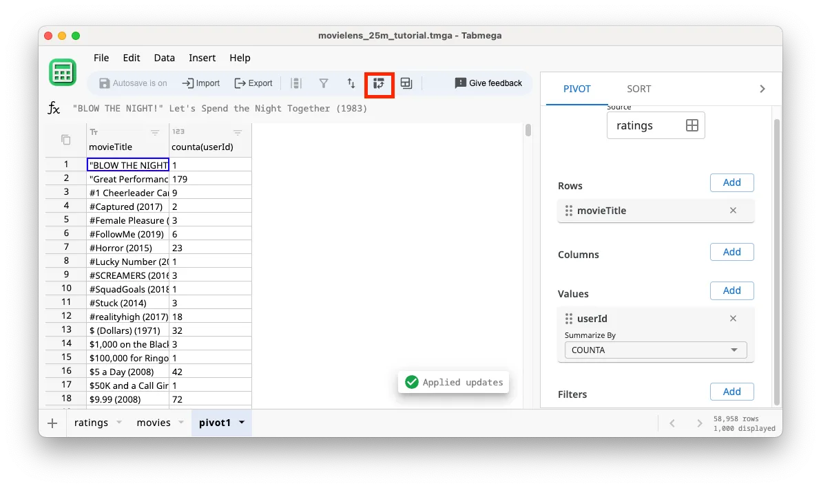
Click on the icon in the blue bar . Alternatively you can use the Insert menu.
-
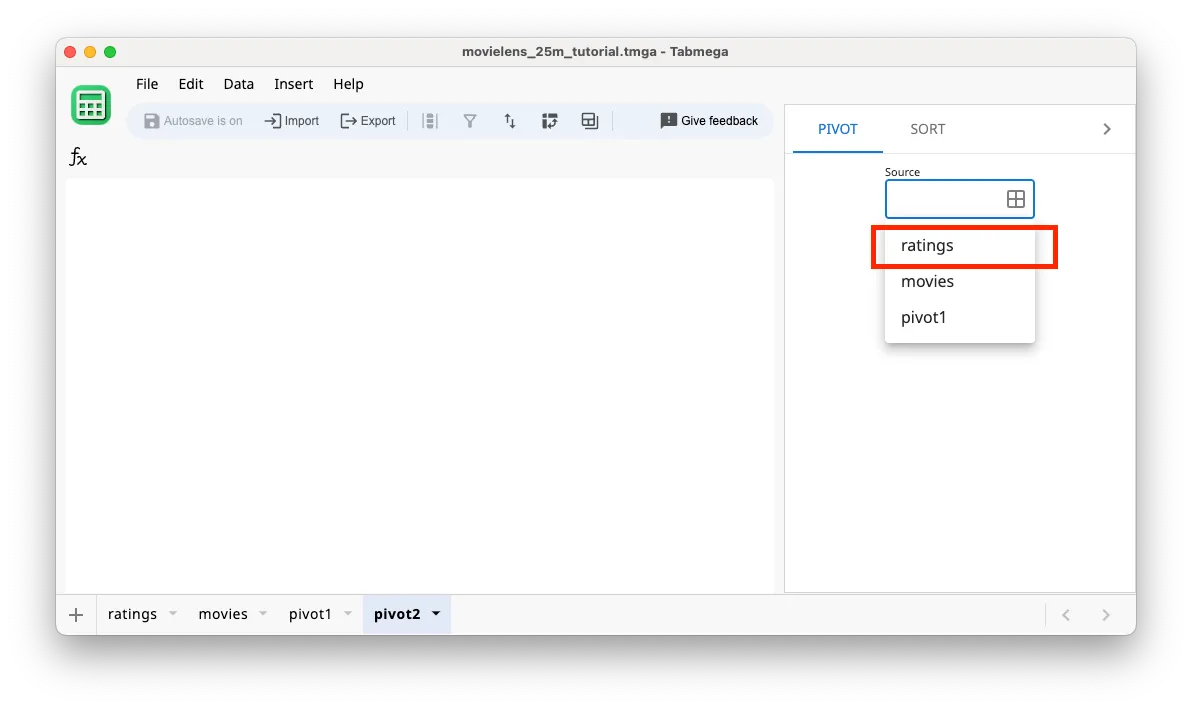
In the pivot2 tab that opens click on Source and select the ratings table as the source.
-
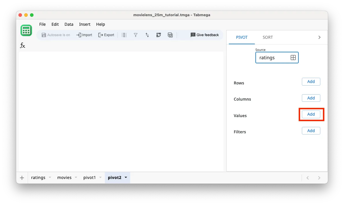
Click on Add button next to Values.
-
Select userID.
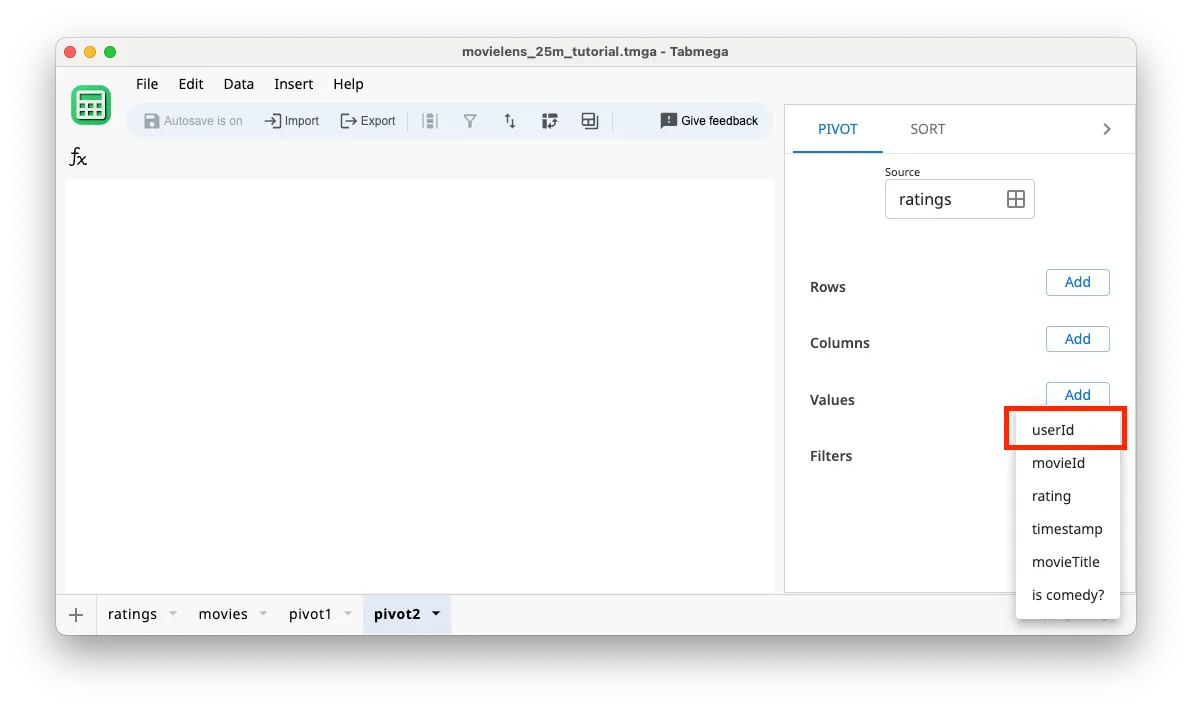
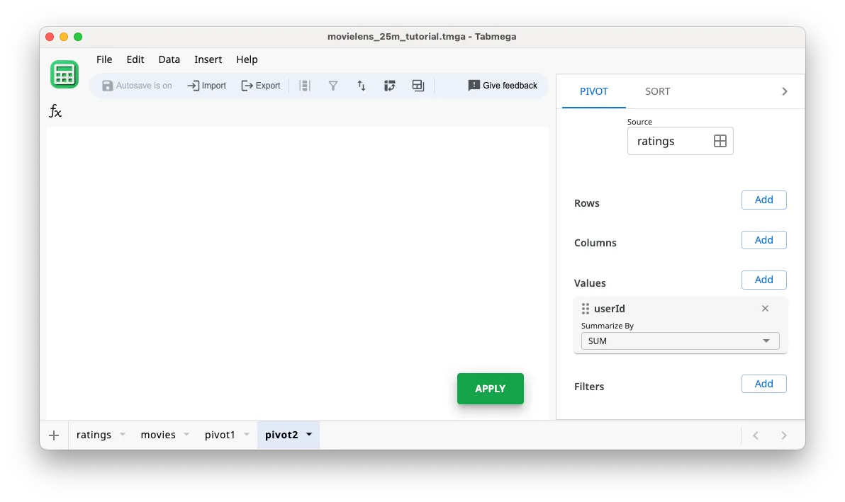
-
For the Summarize By function select
COUNTUNIQUE.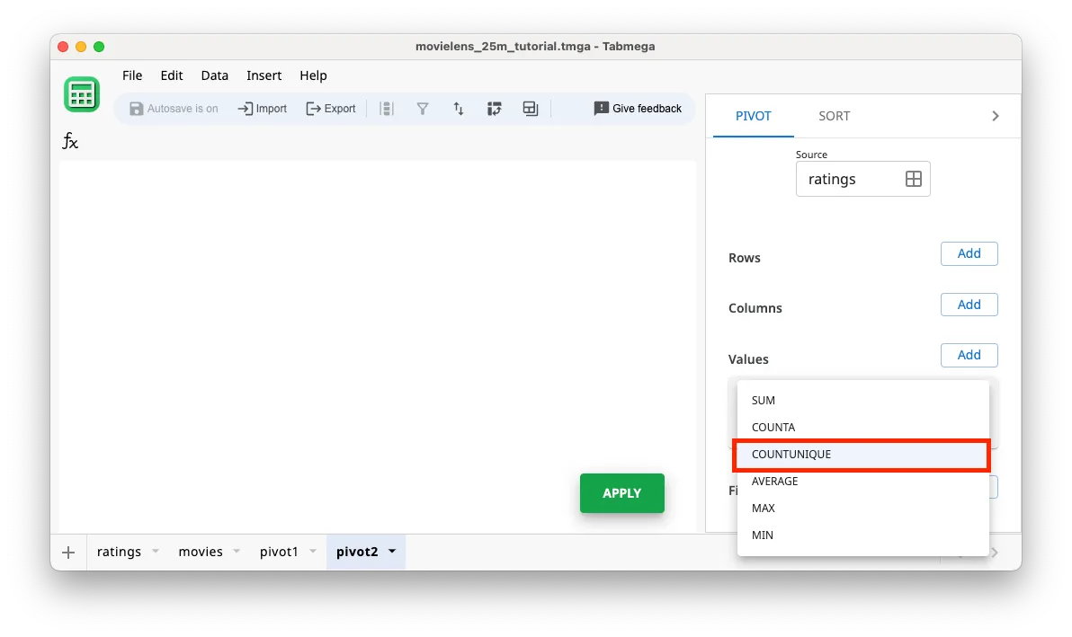
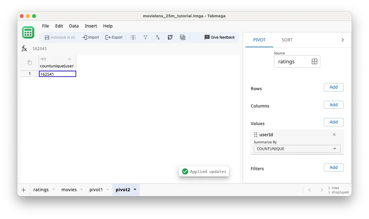
-
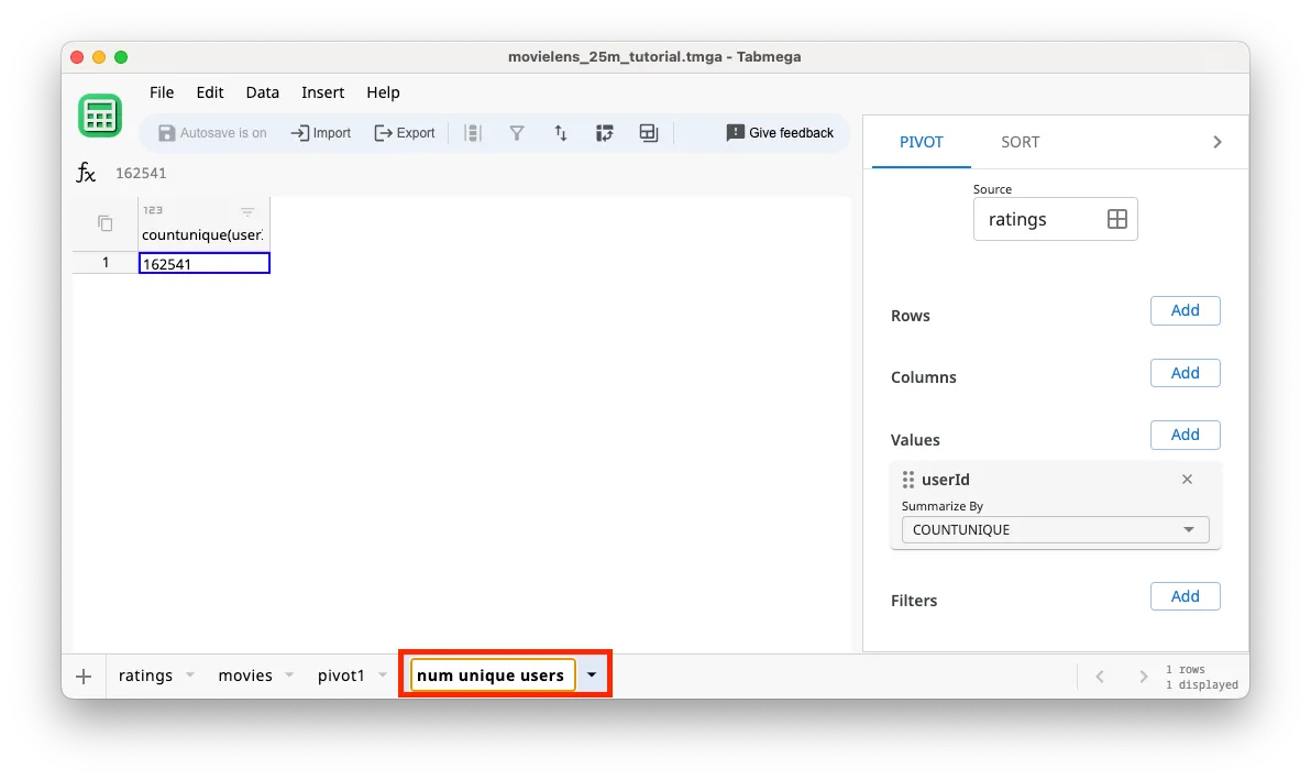
Click on Apply to calculate the result — looks like there are 162,541 unique users in the dataset!
-
[Optional] Let’s rename the tab to num unique users by double clicking on the pivot2 tab and renaming. This makes it easier to navigate to the data when we want it.