Create Pivot Tables

Pivot tables are one of the best features of spreadsheets. Let’s use them in Tabmega.

Adding a pivot table

1. Assuming you are following along from the Filter section of the tutorial, you should be on the ratings table. It’s fine to keep the filter applied for Toy Story (1995) and Jumanji (1995), or to remove the filter. It won’t affect the pivot.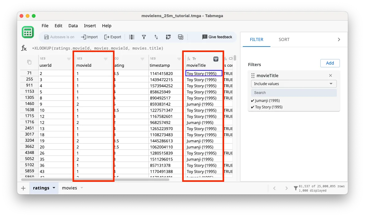
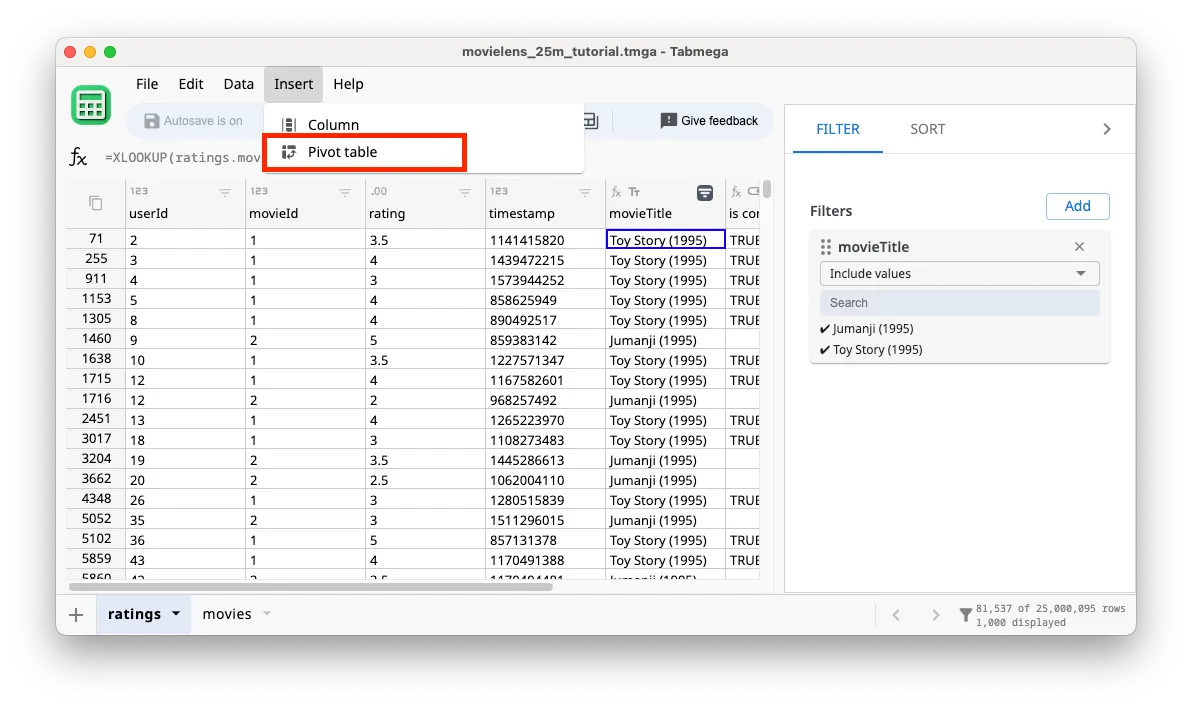
2. Click on the Insert menu at the top of the window, and then Pivot Table.
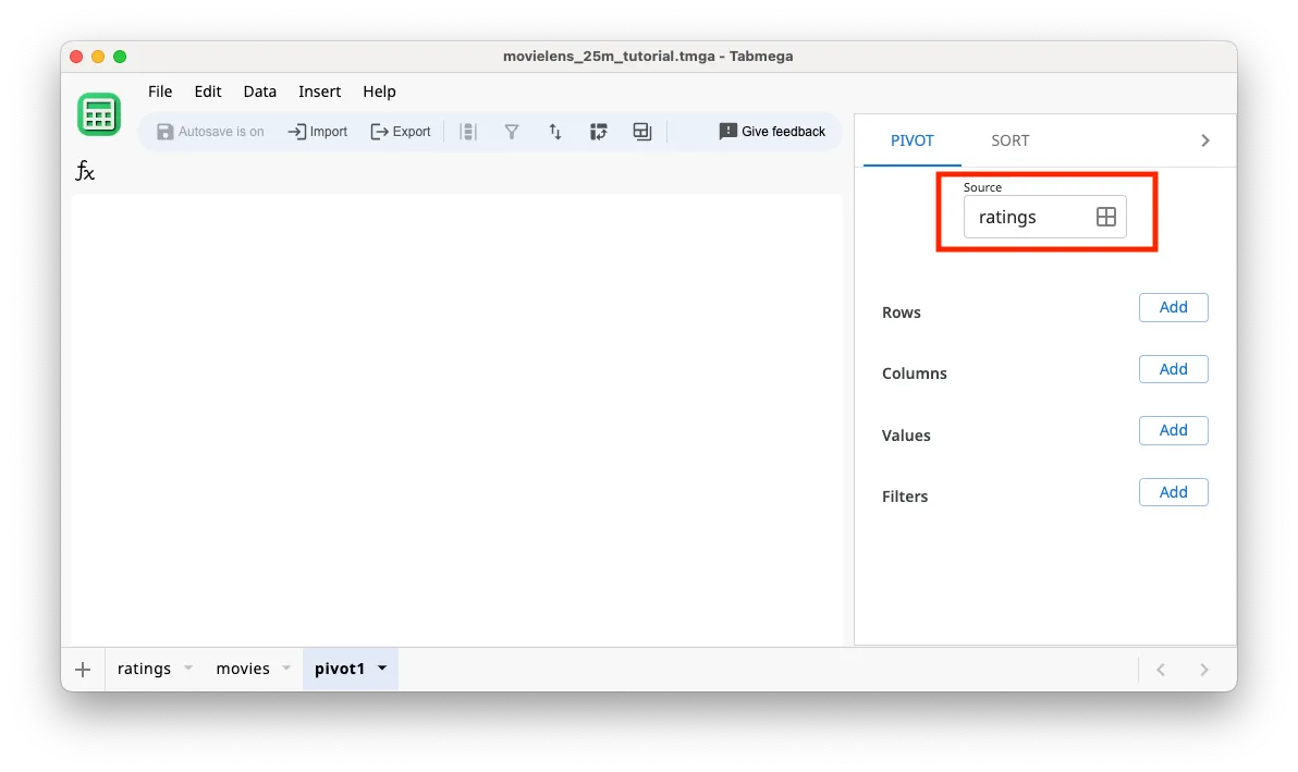
3. You’ll see a new table was created called pivot_1. Ensure that the Source box in the right pivot pane is the ratings table. It should be automatically set to the ratings table if you inserted a pivot while on the ratings table.
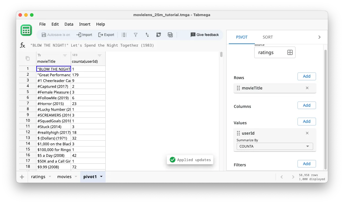
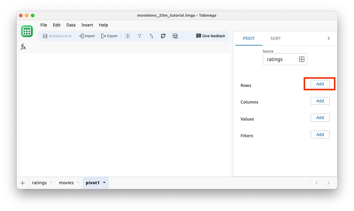
4. Let’s get the count of ratings by movie title. Click on Add button next to Rows.
5. Add movieTitle as a row. It should look like the second screenshot after adding.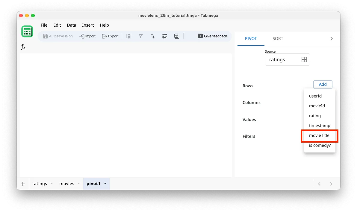
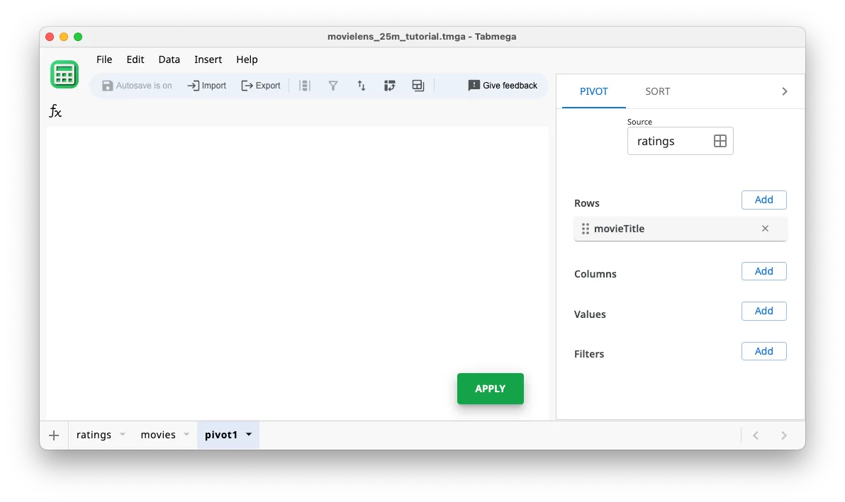
6. Click on Add button next to Values.
7. Add userId as a Value. It should look like the second screenshot after adding.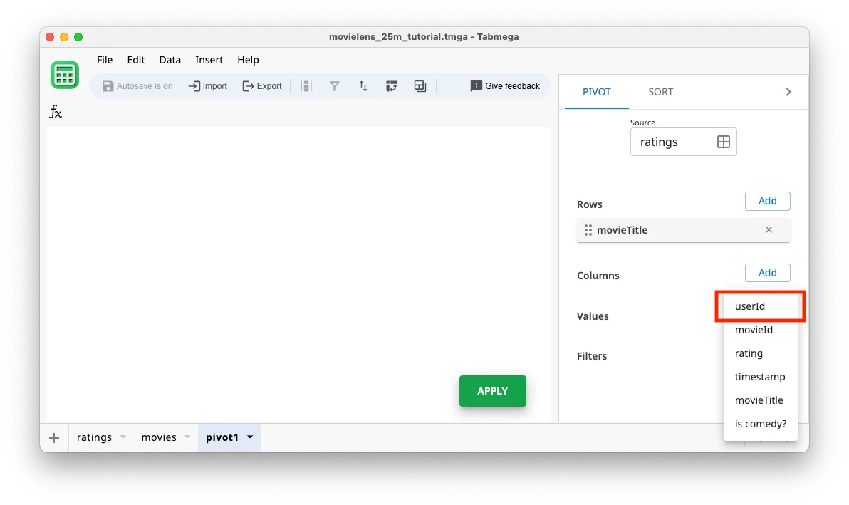
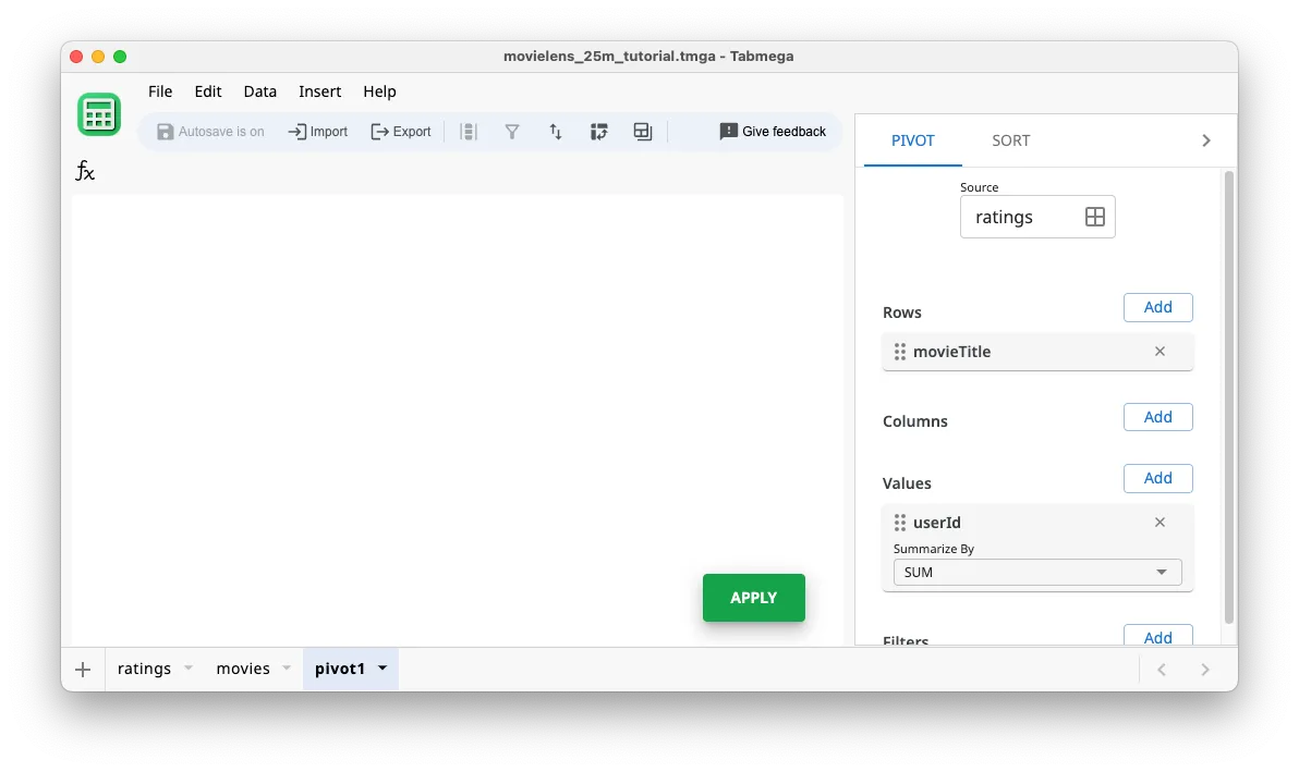
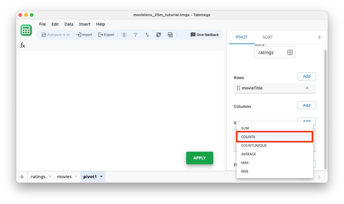
8. By default the Summarize By function is SUM because userId is a numeric value. Update the Summarize By dropdown for userId to be COUNTA which counts non-blanks. There aren’t any duplicate or blank rows, so COUNTA will give the same result as COUNTUNIQUE and will be slightly faster.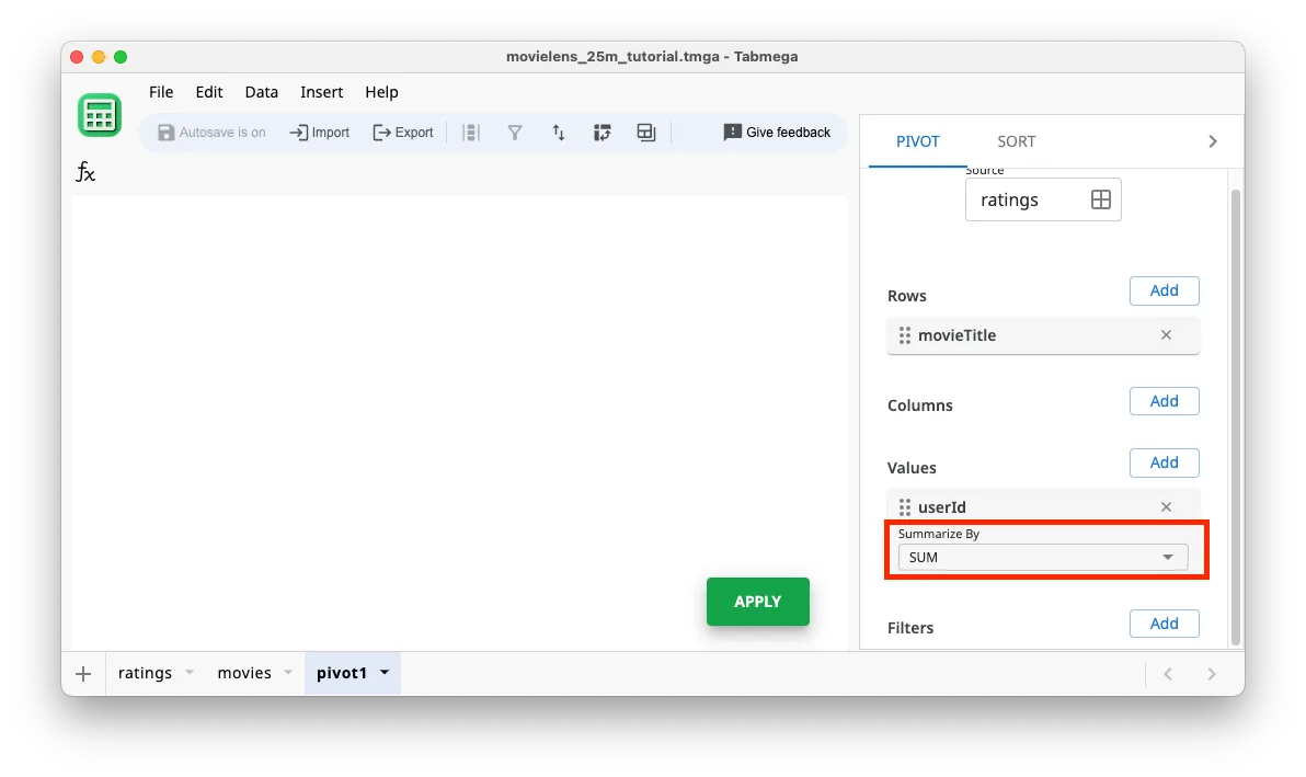
9. As usual, click Apply for the new pivot table to be calculated. Now we can see the number of users that have rated each movie!

Differences from Excel and Google Sheets

In Google Sheets and Excel, you can collapse or expand elements in a pivot table to focus on specific details or hide them, and you can show subtotals and grand totals. In Tabmega, however, pivot tables work a bit differently. They’re always fully expanded, and there are no built-in subtotals or grand totals. This might take some getting used to, but we think there is an advantage: you can easily copy the pivot table results to a new tab and treat it like a regular data table for further analysis (e.g. pivots of pivots, lookups to other tables, etc).

If you’re used to traditional pivot tables, give yourself a little time to adjust. Please give feedback if you really miss the expand,collapse, and subtotal controls.