Use Pivot Results

In this section we’ll learn how to filter our pivot table results and write formulas with them.

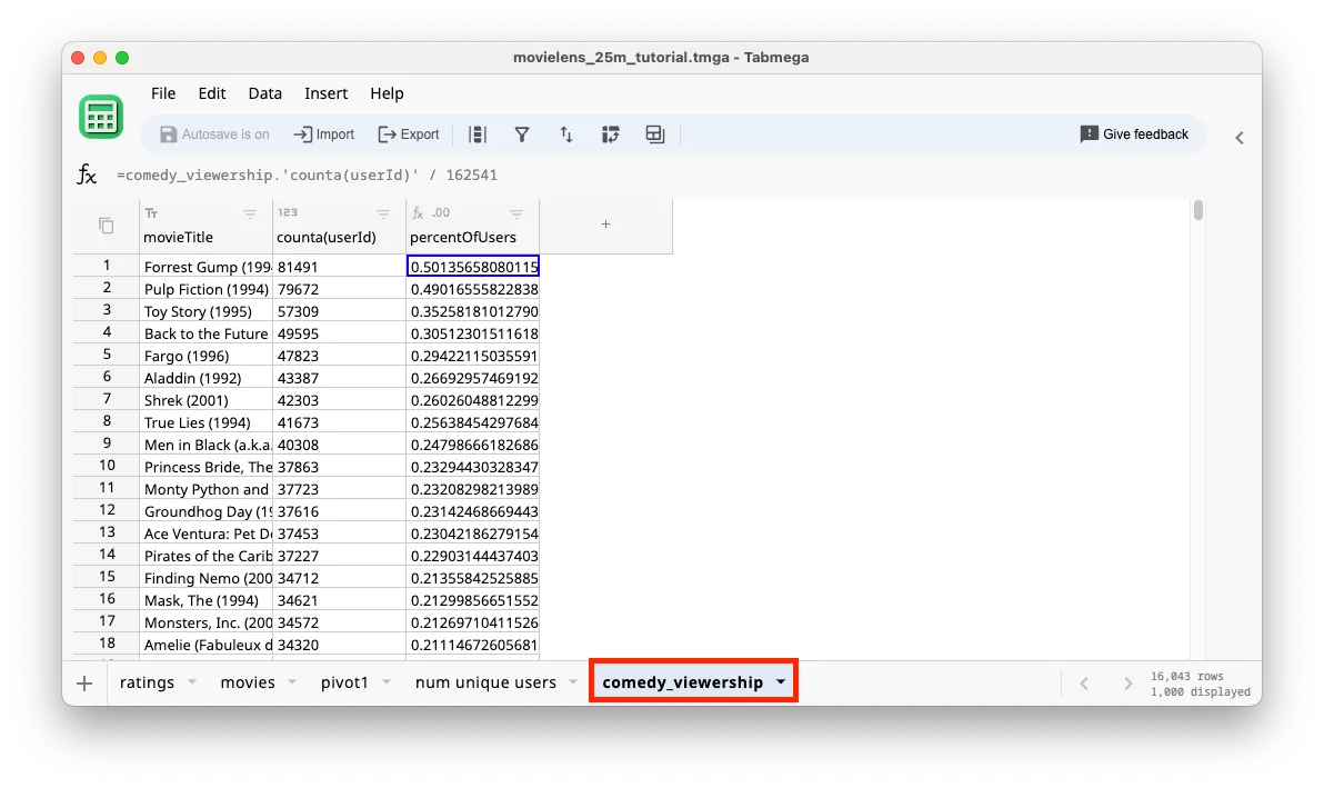
The end output we want is a table that has only comedy movies ordered by number of users descending, with another column that shows the percent of total users that rated the movie like below:

Filter for comedy movies

First let’s update our pivot to filter for comedy movies.

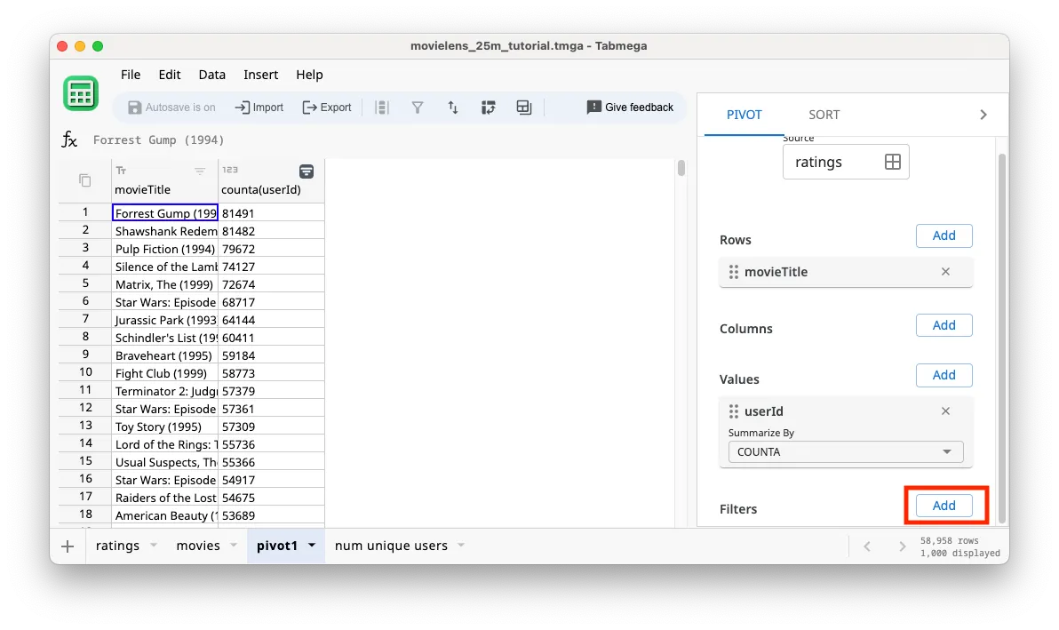
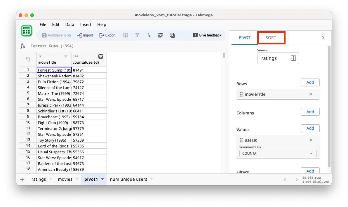
1. Go to the pivot1 tab and click on the Add button next to Filters in the Pivot window.

2. Add is comedy? field.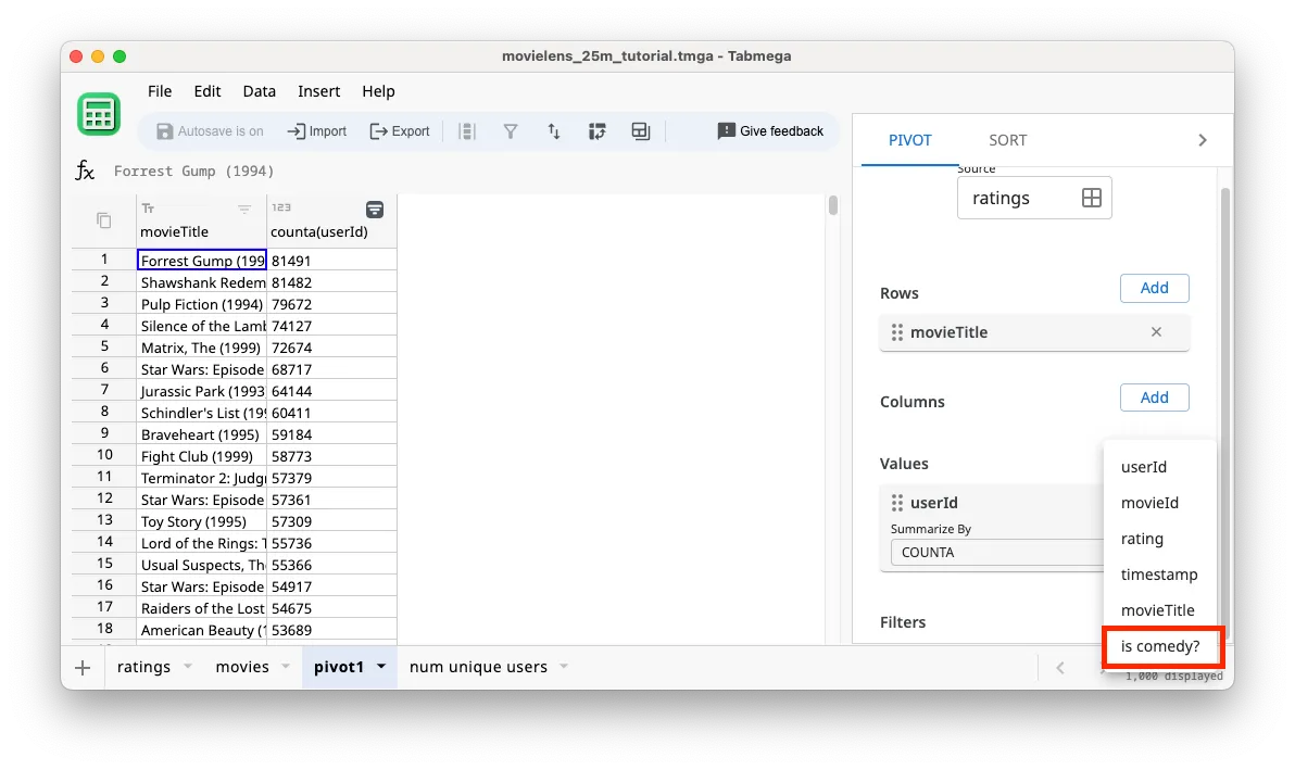

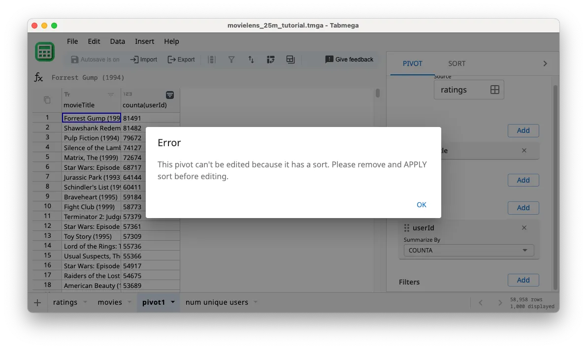
3. You’ll see an error message that we need to remove the Sort from the pivot table in order to edit it.

4. Go to the Sort tab in the right pane.

5. Remove the counta(userId) sort by clicking the X button.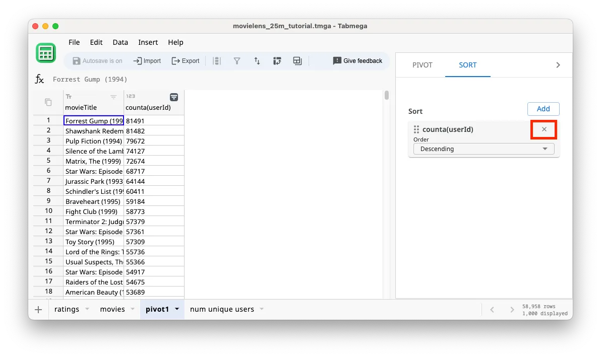

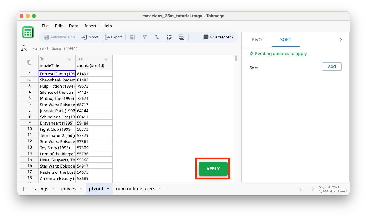
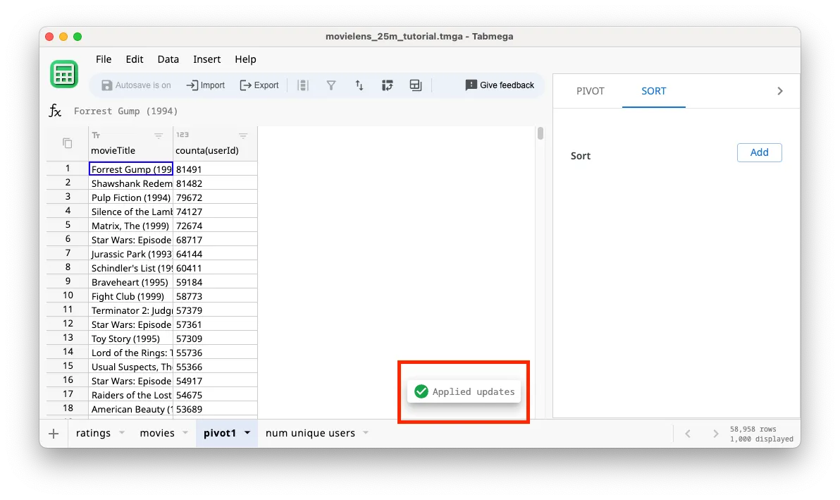
6. Click Apply.

7. You’ll see the processing dialog for a quick second and then you’ll still see the popular movies at the top. This is because removing sorts won’t change the order of a table. You need to apply with new sorts to change the order.

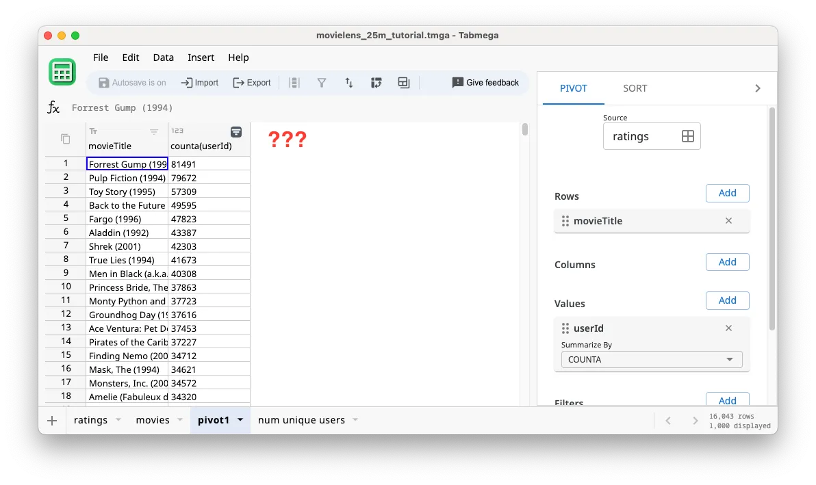
8. Now we can go back to the Pivot tab and add the is comedy? filter.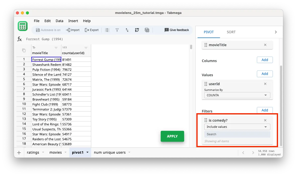

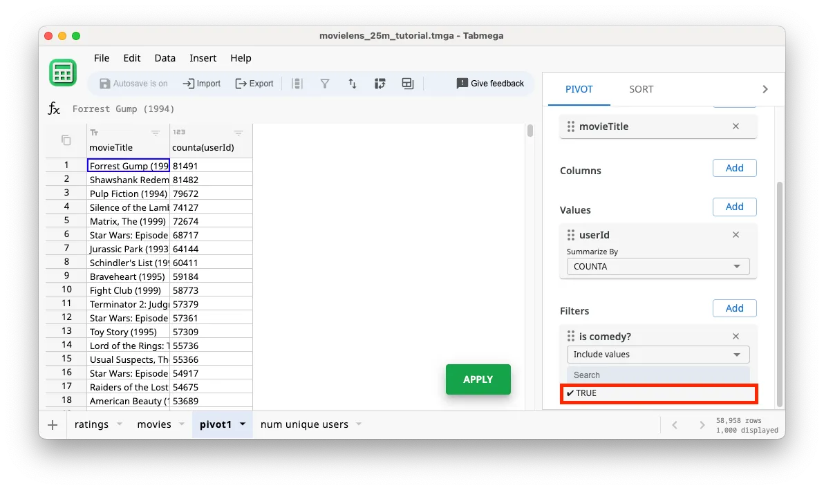
9. Click on the Search box and filter for TRUE.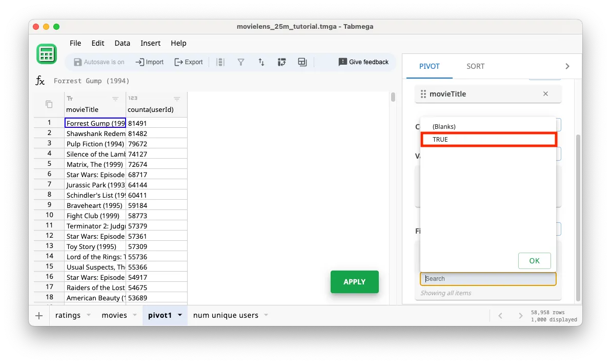

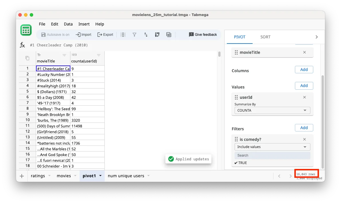
10. As usual, click on Apply to run the calculation. We should see 16,043 rows now instead of ~59K because we are filtering for comedy movies.

11. We lost our ordering of the most popular movies at the top because we recalculated the pivot table. Add the sort back using the steps described in the Sort section. The end result should look like the below screenshot.

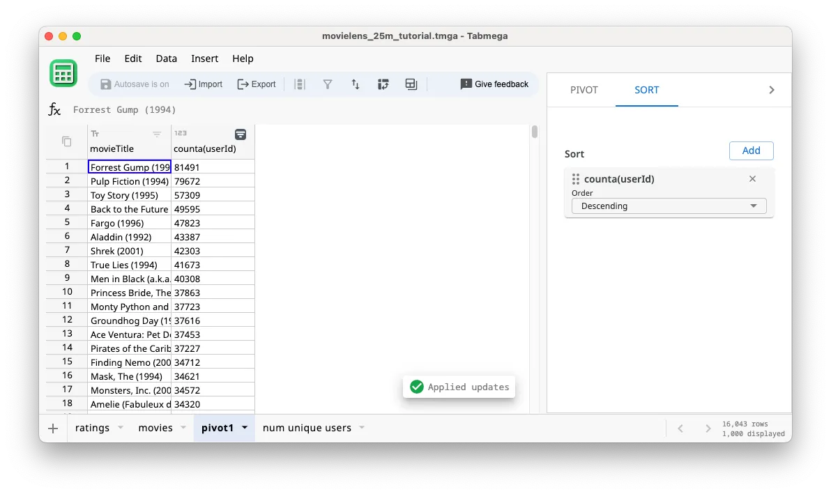
Notice that movies without the Comedy genre tag have disappeared, such as Shawshank Redemption and Silence of the Lambs.

Improvements coming

Expect an improved user experience in February 2024 that will allow editing sorted pivot tables without needing to remove the sort. The current error message helps avoid tricky corner cases, but we will add logic to handle these corner cases in an upcoming release.

Copying pivot values to new table for formulas

We want to insert a calculation column to our pivot table that calculates the percent of total users that have rated the movie. But there is no button to add the column like in the Add Columns and Formulas section.

The solution is simple — we need to copy the pivot values to a new table first. Then we can treat it like a regular data table instead of a pivot table.

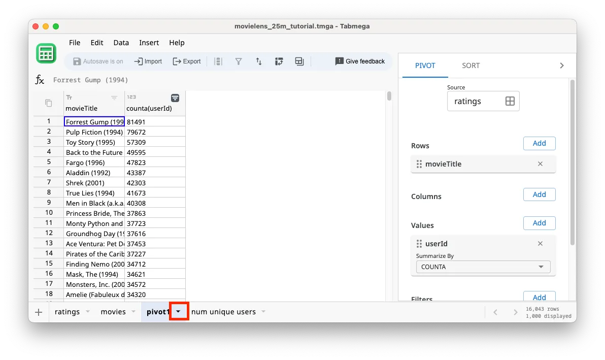
1. Click on the dropdown arrow in the pivot1 tab.

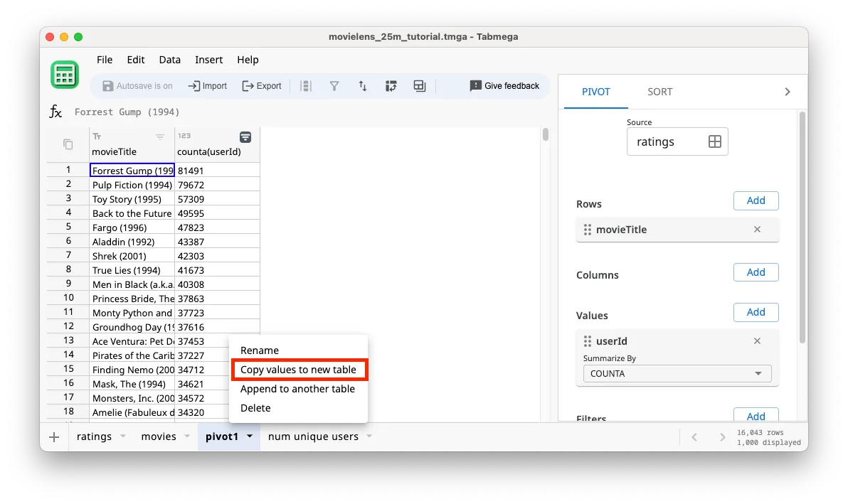
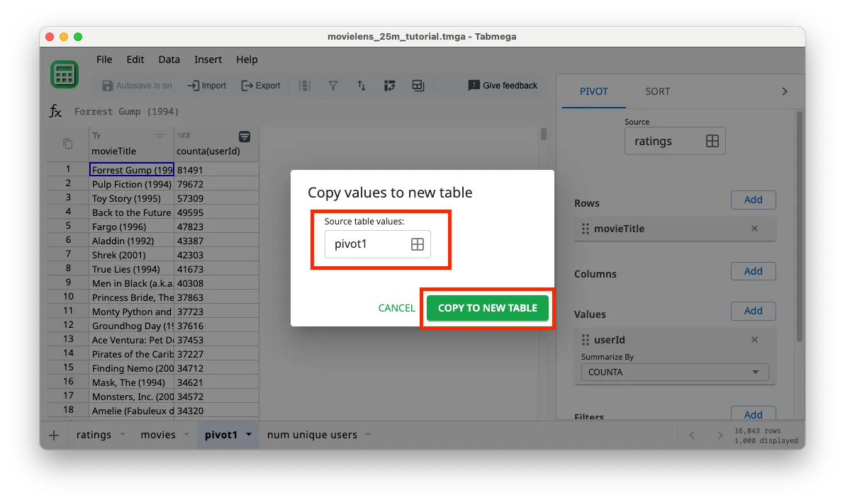
2. Select Copy values to new table.

3. Ensure pivot1 is selected as the Source table, and click COPY TO NEW TABLE.

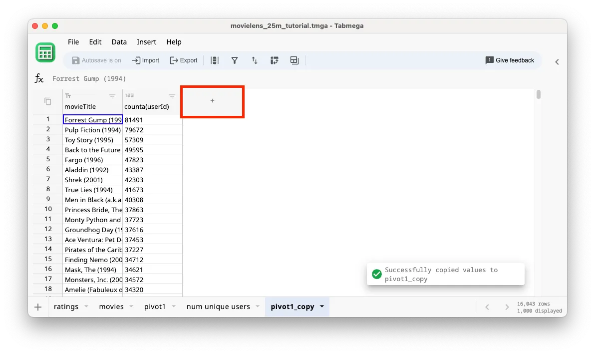
4. In the new pivot1_copy table that was created, you can now click the + button to insert a new column.

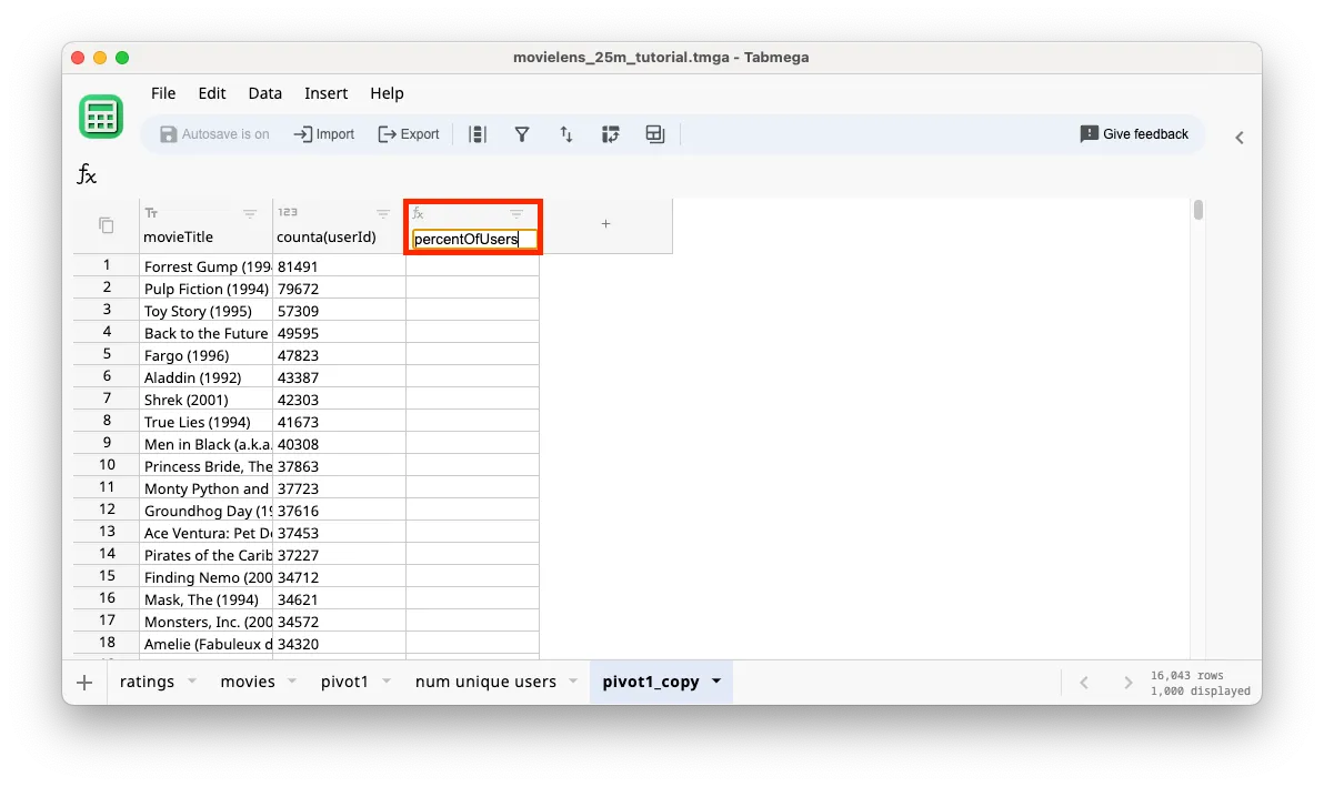
5. Name the new column percentOfUsers.

6. Enter the formula =pivot1_copy.'counta(userId)' / 162541 for the new column. You can use the mouse or keyboard to select the counta(userId) column in the formula as described in Add Columns and Formulas section. 162541 is the result from the num unique users table created in section Sum, Count, Aggregate.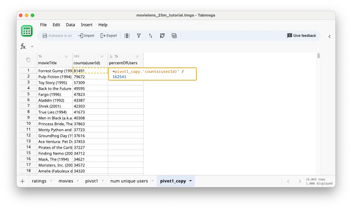

7. As usual, click Apply or Shift+Enter on the keyboard to calculate the new column. We can see that ~50% of users have watched and rated Forrest Gump and Pulp Ficton.

8. [Optional] Let’s rename the table to comedy_viewership so that it is more descriptive of the contents.